Seismic observations on large earthquakes
[Back]
5. Ubiquitous depth-frequency relation of seismic radiation in subduction zones
We investigate global databases of BP images provided by The Incorporated Research Institutions for Seismology (IRIS) over all the Mw 6.5+ earthquakes since 1995. Here, we select 461 earthquakes between 1995 and 2021 within the latitude-longitude range of the available Slab2 plate interface model (Hayes et al., 2018). We then project the HF and LF BP peaks of each earthquake onto the Slab2 model and calculate the corresponding HF and LF centroid depths. The centroid depth is a weighted average of the BP peak depths, the weights being the amplitude of BP peaks. Finally, we select the 245 earthquakes that have a BP centroid depth shallower than 70 km. For most earthquakes, especially the large magnitude ones with a likelihood of better time and spatial resolution of the BP image, we find that the centroid depth of the HF BP peaks is systematically greater than that of the LF peaks. Two events stand out as exceptions: the Mw 9.0 2011 Tohoku-oki earthquake and the Mw 8.3 2006 Kuril Island earthquake. For the 2011 Tohoku-oki earthquake, the exception is due to the different choice of frequency bands by the IRIS database, and we have shown that the refined BP results clearly present the depth-frequency relation.
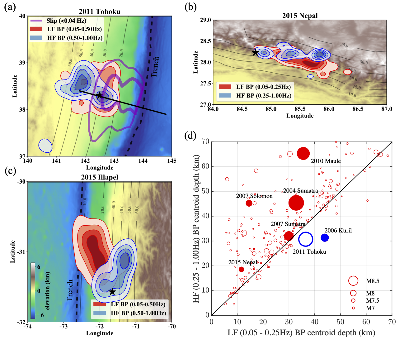
Ubiquitous depth-frequency relation found by back-projection observations. (a)-(c) BP images of the Mw 9.0 2011 Tohoku-oki, the Mw 7.9 2015 Gorkha, and the Mw 8.3 2015 Illapel earthquakes, respectively. The BP images are reconstructed using the imCS-BP method developed by Yin et al. (2018), and only the contours of 20%, 40%, 60%, and 80% maximum power are shown. The dashed black lines indicate the trench. The thin gray contours show the Slab2 model (Hayes et al., 2018). The purple contours in (a) show the 20 m and 50 m of coseismic slip distribution during the 2011 Tohoku earthquake from Lay et al. (2012), and the black solid line shows the location of the velocity profile of Miura et al. (2005). (d) Centroid depths of the low-frequency (0.05 - 0.25 Hz) BP images compared with the high-frequency (0.25 - 1 Hz) BP images from 245 M > 6.5 earthquakes.
4. Global patterns of STF complexity
We developed different metrics to look at the complexity patterns of earthquake source time functions (STFs) in the global database (specifically SCARDEC database):
(1) DTW clustering
We develop a dynamic time warping (DTW) clustering method to focus on the STF general shapes. We use the dynamic time warping (DTW) distance and hierarchical clustering to group earthquakes based on the general shape of their STFs. The clusters exhibit different degrees of STF shape complexity, as measured by the number of prominent peaks (G1-G4). The clustering also indicates an association between the degree of STF complexity (or group) and earthquake source parameters. We have already submitted our finished manuscript to AGU Advances, and the pre-print can be found here.
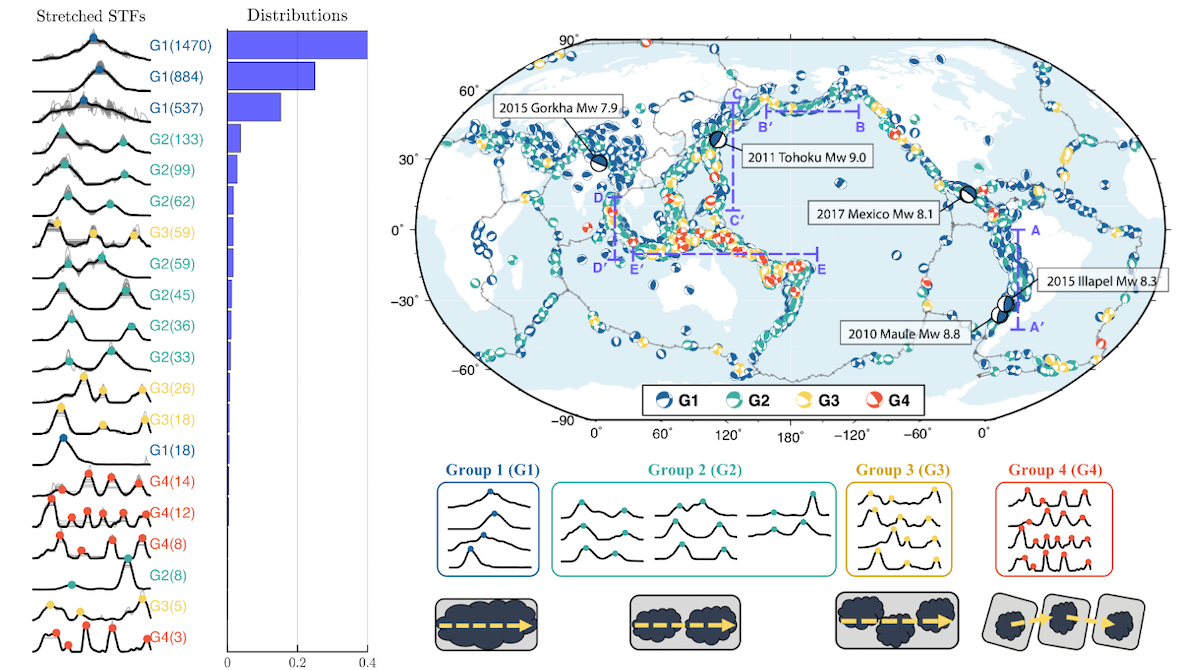
(Left) SCARDEC STFs after DTW stretching and clustering. Here STF complexity is quantified by the number of prominent peaks into 4 groups. (Right top) Global distribution of STF complexity. (Right bottom) Schematic illustribution of rupture inferred from STF compleixty.
(2) Gaussian-subevent decomposition
Different from the DTW clustering, which focuses on the patterns of STF general shapes , we also decompose the STF as a sum of “subevents” that are Gaussian pulses. We iteratively perform the subevent decomposition from onset of rupture (time zero): searching for the best-fit Guassian pulse for the first peak, then subtracting that Gaussian subdevent from the STF, repeating this for the residual until no obvious peaks can be found. In this way, we can quantify the STF complexity with the number and magnitudes of those subtracted Gaussian subevents. A very clear scaling pattern has been found between the main event magnitude and corresponding subevent magnitudes. Applying this to early magnitude estimates, we show that the main event magnitude can be estimated after observing only the first few subevents (here for more details please).
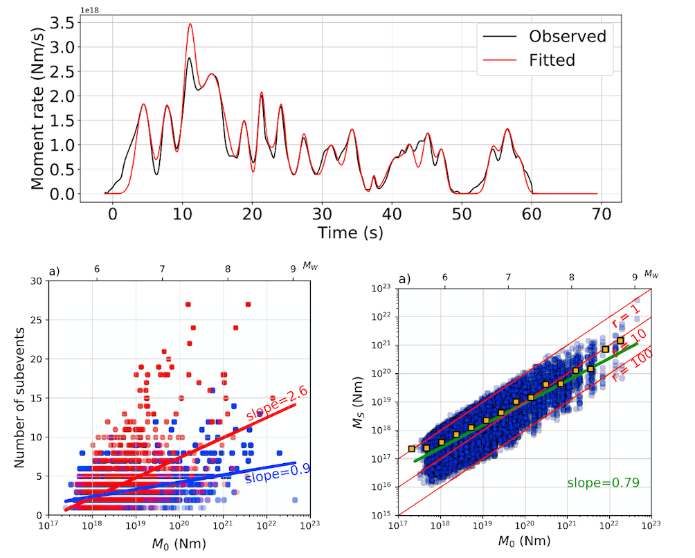
(Top) Example of Guassian-subevent decomposition for STF. (bottom) Scaling relations found for SCARDEC STF database: main event seismic moment (M0) vs Number of subevents; main event seismic moment (M0) vs subevent seismic moment (Ms)
3. Backprojection resolution from the theoretical formulation
Based on the theoreitcal formulation of linear back projection (see here), the resolution matrix F(ω) only depends on source mechanism and source-receiver geometry, we can further calculate the resolvability, which is defined as the 2D correlation coefficient between the resolution matrix and an identity matrix, and use it to evaluate the BP resolutions for real seismic array-source configurations. For more details, please see Yin and Denolle (2019 GJI).
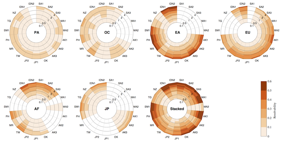
BP resolvability for most of the seismic arrays in the world. The higher resolvability implies better BP resolution for a specific seismic array towards a seismic region.
2. Combination of Backprojection (BP) and Spectral analysis (SP) to infer the spatial and temporal evolution of earthquake rupture
We develop a methodology that combines the backprojection (BP) and source spectral analysis (SP) of teleseismic P waves to provide metrics relevant to earthquake dynamics of large events. We improve the compressive sensing backprojection (CS-BP) method (Yao et al., 2011; Yin & Yao, 2016) by an auto-adaptive source grid refinement as well as a reference source adjustment technique to increase spatial and temporal resolution of the locations of the radiated bursts. We also use a two-step source spectral analysis based on (i) simple theoretical Green’s functions that include depth phases and water reverberations and on (ii) empirical P-wave Green’s functions. Furthermore, we propose a source spectrogram methodology that provides the temporal evolution of dynamic parameters such as radiated energy and falloff rates. Combination of BP and SP analysis provides a spatial and temporal evolution of these dynamic source parameters and is an attempt to bridge kinematic observations with earthquake dynamics. For more details, please see Yin et al. (2018 JGR).
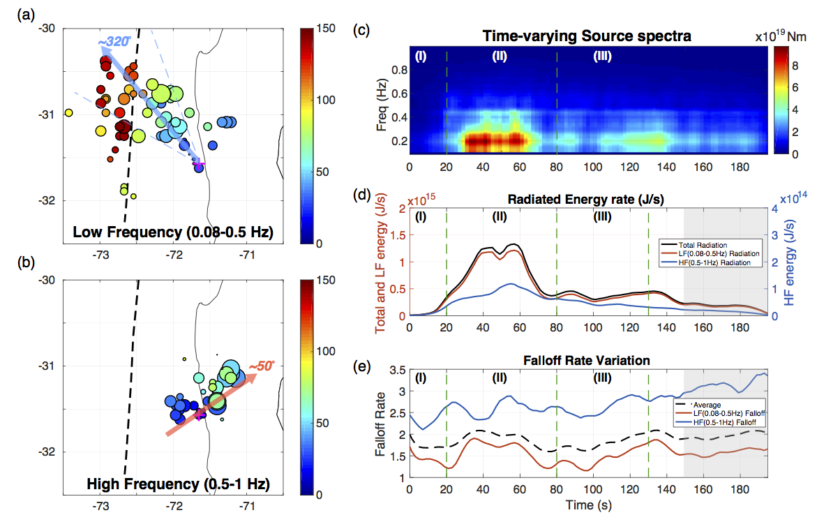
Observations on the 2015 Illapel earthquake: (a) low frequency data (0.08-0.5Hz) BP results. (b) high frequency (0.5-1Hz) BP results. Size and color of circles corresponds to the relative amplitude and source time, respectively. (c) Recovered source spectra in the time-frequency space. (d) and (e) Temporal variations of radiated energy and spectral falloff rate in both low and high frequency bands, respectively. Published in Yin et al. (2018)
1. Compressive Sensing BackProjection imaging on the rupture process of large earthquakes
Compressive Sensing BackProjection (CSBP), which is first developed by Yao et al. (2011), is a high resolution backprojection method in frequency domain. CSBP applies the sparsity inversion with L1-norm based on the theory of compressive sensing. Compared with other types of backprojection methods, one of the key advantages of CSBP is that it can get high-resolution images in both high- and low-frequency bands. We improve this method in both efficiency and resolution, and further applied to some recent large earthquakes: 2012 Sumatra Mw8.6 earthquake; 2015 Gorkha Mw 7.8 earthquake; 2015 Illapel Mw8.3 earthquake. From our results of all those events, we found a common frequency-dependent pattern that the high-frequency and low-frequency results are at different part on the fault. Those observations directly shows the heterogeneity on the coseismic fault interface, and implies the different physics behind the high-frequency and low-frequency seismic radiation.
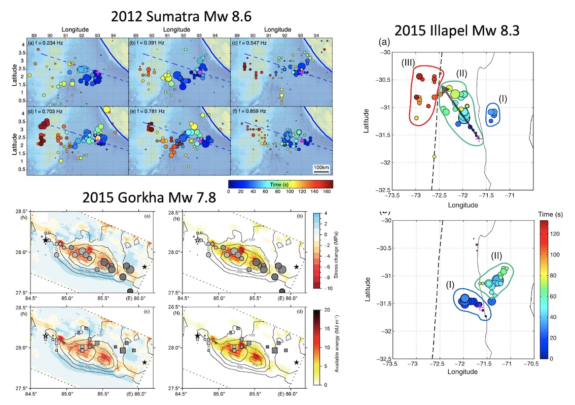
CSBP results of 2012 Sumatra Mw8.6 earthquake; 2015 Gorkha Mw 7.8 earthquake; 2015 Chile Mw8.3 earthquake in different frequency bands. Dots color shows the time. Please refer to the papers for details of results and explanations.
[Back]